


Overview
This is the second article of Demystifying Machine Learning series, frankly, it is basically the sequel of our previous article where we explained Linear Regression using Normal equation. In this article we'll be exploring another optimizing algorithm known as Gradient Descent, how it works, what is a cost function, mathematics behind gradient descent, Python implementation, Regularization and some extra topics like polynomial regression and using regularized polynomial regression.
How Gradient Descent works (Intuition)
Gradient descent is basically an iterative optimizing algorithm i.e. we can use it to find the minimum of a differential function. Intuitively we can think of a situation where you're standing somewhere on a mountain and you want to go to the foot of that mountain as fast as possible. Since we're in a random position on the mountain, one way is to move along the steepest direction while taking small steps (taking large steps towards steepest direction may get you injured) and we'll see later that taking large steps is also not good for algorithm too.
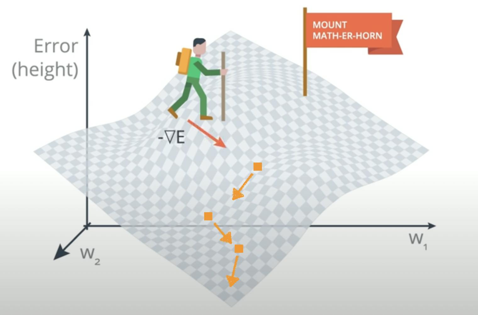
Now that's something similar we are going to do for optimizing our hypothesis to give the least error. As we learnt in the previous article that we need to find the optimal parameters θ, that helps us to calculate the best possible hyperplane to fit the data. In that article, we used the Normal equation to directly find those parameters but here that's not gonna happen.
We are randomly going to pick the parameters and then calculate the cost function that will tell us how much error those random parameters are giving, then we use gradient descent to find the minimum of that cost function and optimize those random parameters into the optimal ones.
Cost Function
A cost function is basically a continuous and differentiable function that tells how good an algorithm is performing by returning the amount of error as output. The lesser the error, the better the algorithm is doing that's why we randomly generate the parameters and then keep changing them in order to reach the minimum of that cost function.
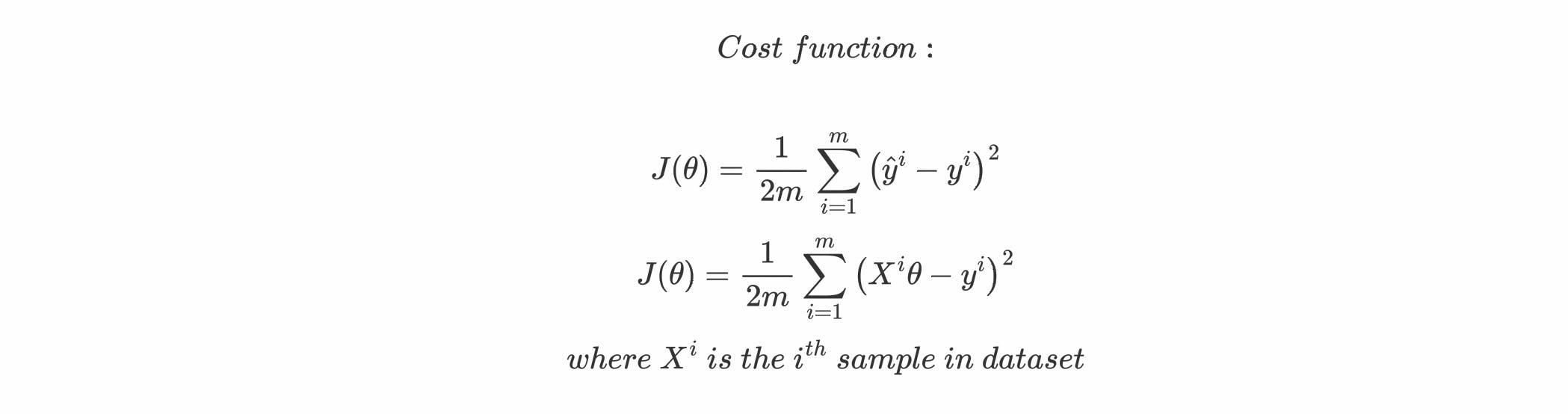
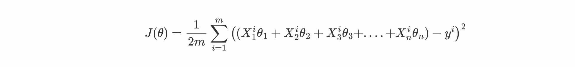
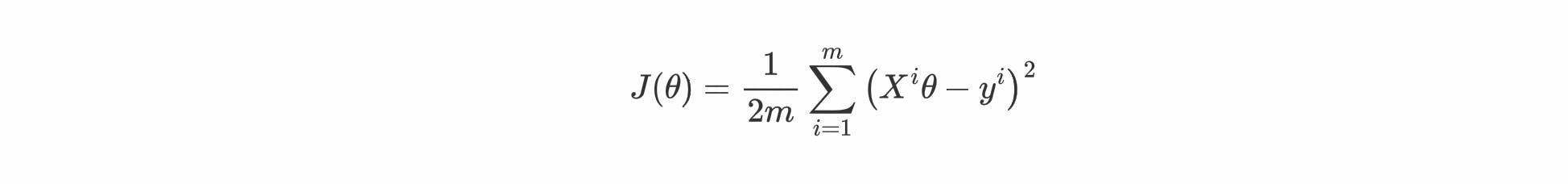
Now let's define the cost function for Linear regression. First, we need to think that in linear regression how we can calculate the error. Mathamtically error is the difference between the original value and the calculated value. Luckily we can use this definition here. Our original values are the target matrix itself and the calculated values are the predictions from our hypothesis.
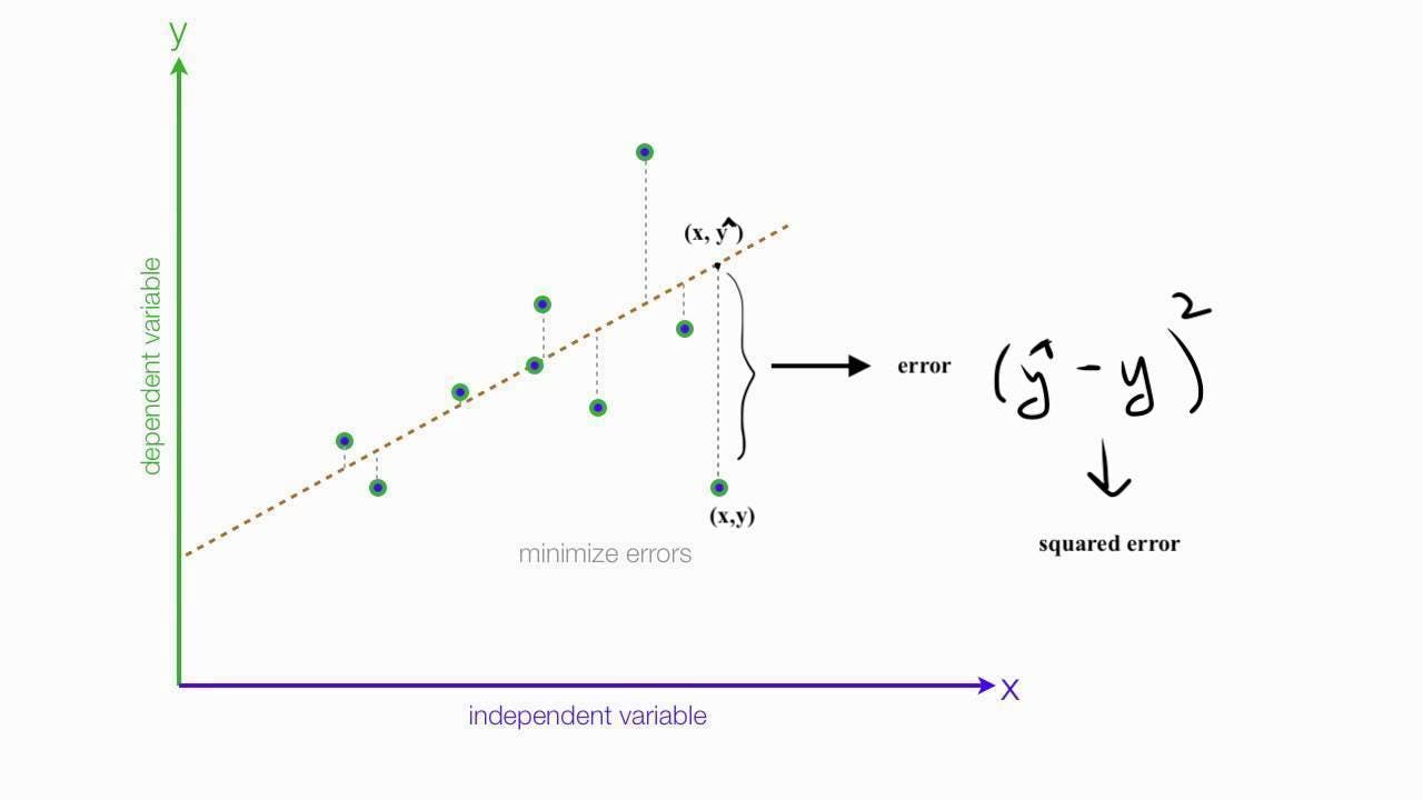
We simply subtract the original target value from the predicted target value and take the square of them as the error for a single sample. Ultimately we need to find the squared error for all the samples in the dataset and take their mean as our final cost for a certain hypothesis. Squaring the difference helps in avoiding the condition when the negative and positive errors nullify each other in the final hypothesis's cost.
This error function is also known as Mean Square Error (MSE).
So mathematically let's say we have m number of samples in the dataset then:
It's important to notice that our cost function J(θ) is depend upon the parameters θ because our y(target) and X are fixed, the only varying quantity are the parameters θ and it makes sense because that's how gradient descent will help us in finding the appropriate parameters for a minimum of the cost function.
Mathematics of Gradient Descent
Time to talk Calculus.
Before diving into the algorithm let's first talk about what is a Gradient?
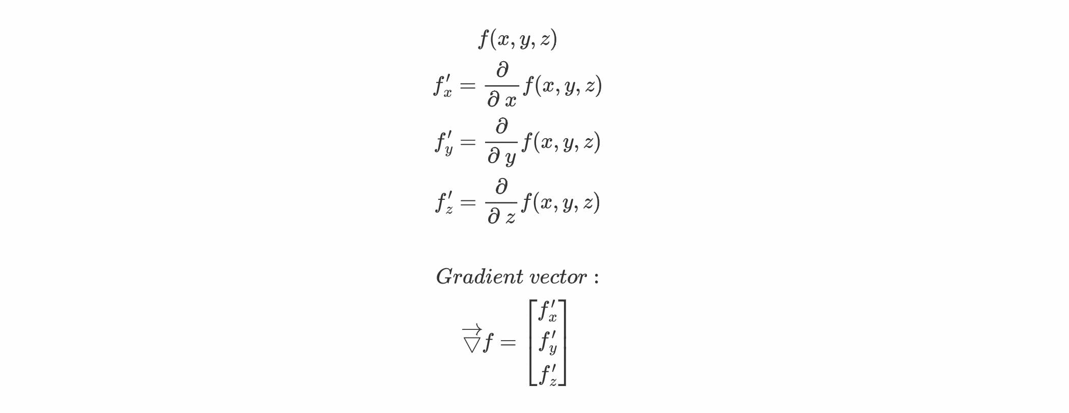
Gradient of a differentiable function is a vector field whose value at a certain point is a vector whose components are the partial derivatives of that function at that same point. Alright so many big words let's break them down and try to understand what it really is?
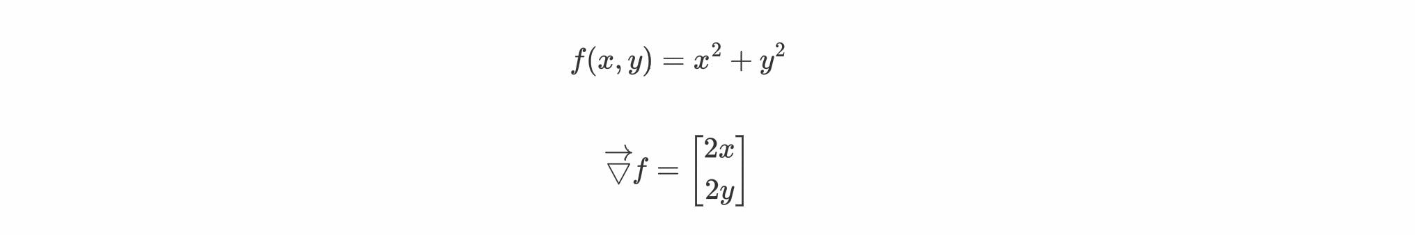
Mathematically suppose you have a function f(x,y,z) then the gradient at some point will be the vector whose components are going to be the partial derivatives of f(x,y,z) w.r.t to x,y and z at that point.
Property: At a certain point, the gradient vector always points towards the direction of the greatest increase of that function.
Since we need to go in the direction of greatest decrease that's why we follow the direction of negative of the gradient vector.
Gradient vector is always perpendicular to the contour lines of the graph of a function (we'll be dealing Contour graphs later)
Let's visualize the gradient concept using graphs. Say a function f(x,y) as:
If we plot the above graph, it'll look something like this:
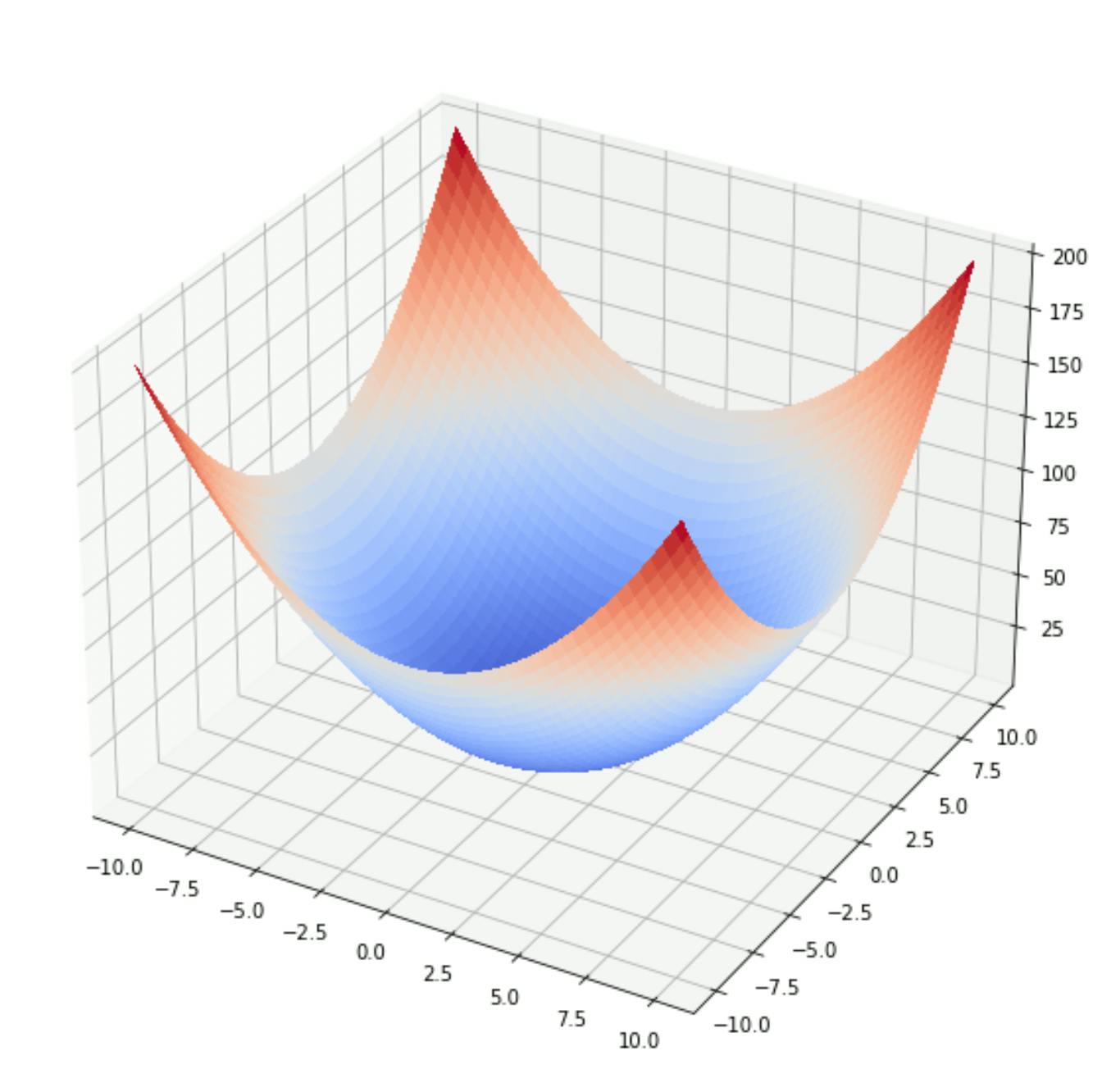
If you're aware of vector calculus, then you probably know that Contour plots are very useful for working with 3D curves. A contour plot is basically a 2D graph that is the sliced version of a 3D plot along the z-axis at regular intervals, so if we graph the Contour plot of the above function then it'll look something like:
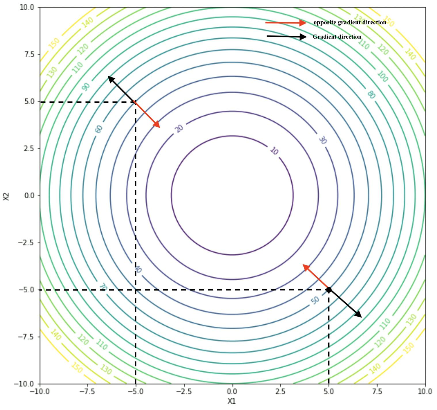
Now, this graph makes it really clear that gradient always points in the direction of the greatest increase of the function, as we can see that the black arrows represent the direction of the gradient and the red arrow represent the direction where we need to move in our cost function to reach the minimum.
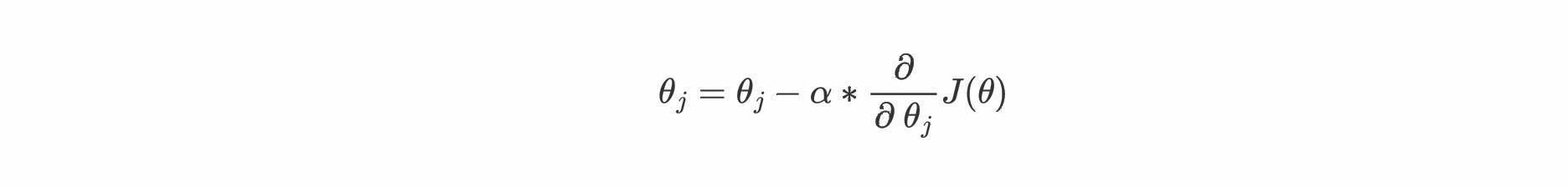
Great now we know that in order to reach the minimum we need to move in the opposite direction of the gradient that is in the -∇f(θ) direction and keep updating our initial random parameters accordingly.
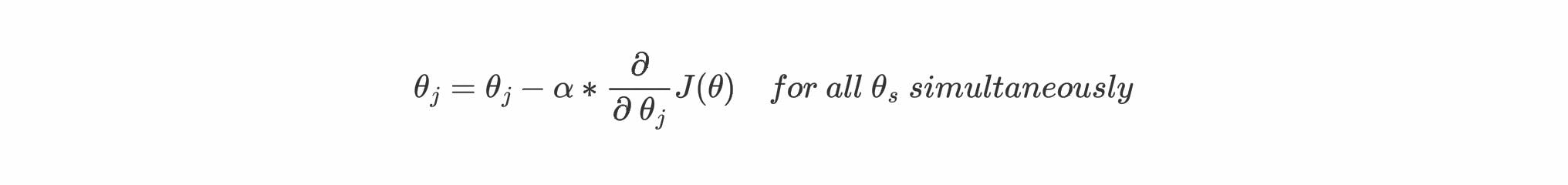
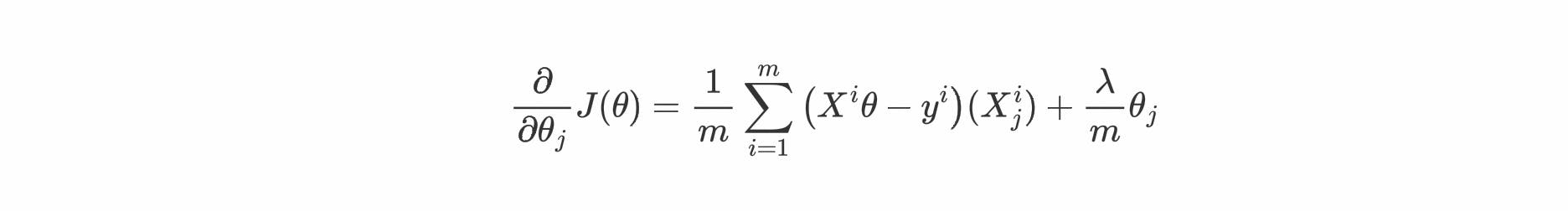
- θ is the matirx of all parameters θs
- θj is the parameter for jth feature
- J(θ) is the cost function
- α is learning rate
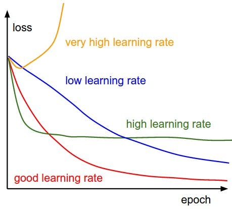
Everything seems obvious instead of this symbol α . It's known as learning rate, remember we discussed that we need to take small steps, α makes sure that our algorithm should take small steps for reaching the minimum. The learning rate is always less than 1.
But what if we keep a large learning rate?
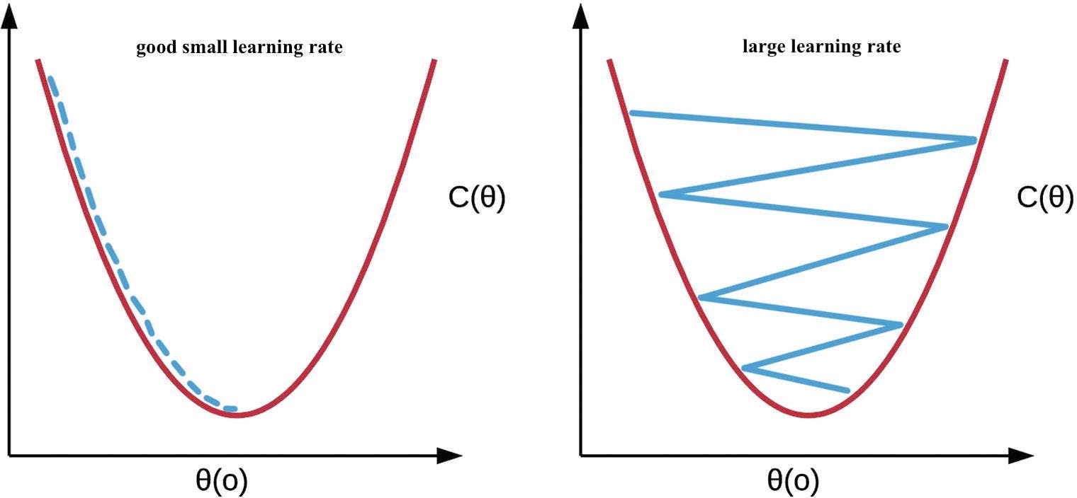
As we see in the above figure that our cost function will not able to reach a minimum if we take large learning rates and its results in an increment of loss instead of decreasing it as represented below.
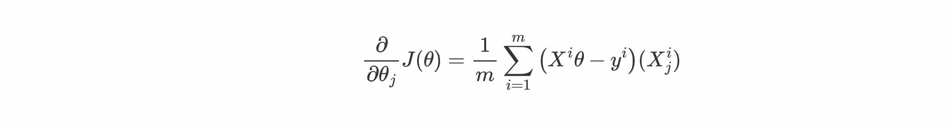
Applying Gradient descent to cost function
In this section, we'll be deriving the formulas for gradients so that we can directly use those formulas in Python implementation. Since we already have our cost function as:

expanding Xi into individual n features as [Xi1, Xi2, Xi3, ....., Xin ] then:
This form will be easier to understand the calculation of gradients, let's compute them for each θj.
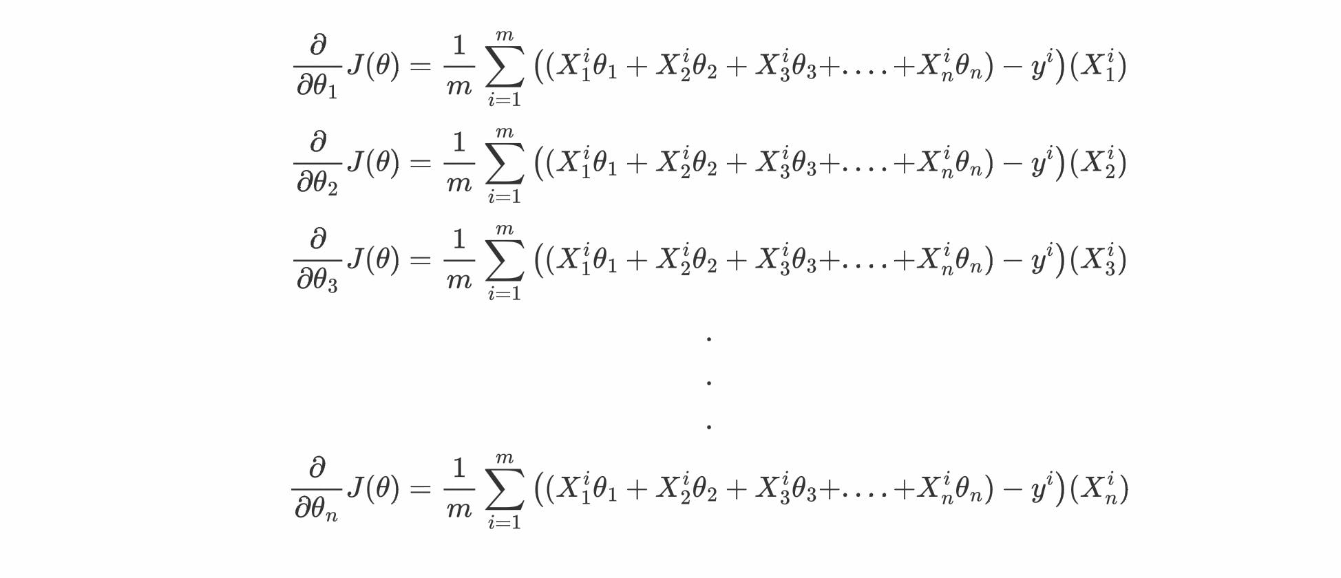
so basically we can write the partial derivative of cost function w.r.t to any θj as :
Now we can loop over each θj from 0 to n and update them as :
Note: θ0 represent the bias term
That's great, now we have all the tools we need let's jump straight into the code and implement this algorithm in Python.
Python Implementation
In this section, we'll be using Python and the formulas we derived in the previous section to create a Python class that will be able to perform Linear Regression by using Gradient Descent as an optimizing algorithm to work on a dataset.
*Note: All the code files can be found on Github through this link.*
And it's highly recommended to follow the notebook along with this section for better understanding.
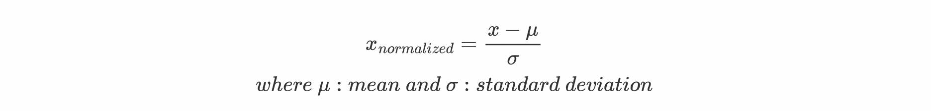
Before we dive into writing code one important observation is to keep in mind that before using gradient descent, it's always helpful to normalize the features around its mean. The reason is that initially in the dataset we can have many independent features and they can have way different values, like on average number of bedrooms can be 3-4 but the area of the house feature can have way large values. Normalizing makes all the values of different features lie on a comparable range and it also makes it easier for the algorithm to identify the patterns.
class LinearRegression:
    def __init__(self) -> None:
        self.X = None
        self.Y = None
        self.parameters = None
        self.cost_history = []
        self.mu = None
        self.sigma = None

    def calculate_cost(self):
        """
        Returns the cost and gradients.
        parameters: None

        Returns:
            cost : Caculated loss (scalar).
            gradients: array containing the gradients w.r.t each parameter

        """

        m = self.X.shape[0]

        y_hat = np.dot(self.X, self.parameters)
        y_hat = y_hat.reshape(-1)
        error = y_hat - self.Y

        cost = np.dot(error.T, error)/(2*m) # Modified way to calculate cost

        gradients = np.zeros(self.X.shape[1])

        for i in range(self.X.shape[1]):
            gradients[i] = np.mean(error * self.X[:,i])

        return cost, gradients


    def init_parameters(self):
        """
        Initialize the parameters as array of 0s
        parameters: None

        Returns:None

        """
        self.parameters = np.zeros((self.X.shape[1],1))


    def feature_normalize(self, X):
        """
        Normalize the samples.
        parameters:
            X : input/feature matrix

        Returns:
            X_norm : Normalized X.

        """
        X_norm = X.copy()
        mu = np.mean(X, axis=0)
        sigma = np.std(X, axis=0)

        self.mu = mu
        self.sigma = sigma

        for n in range(X.shape[1]):
            X_norm[:,n] = (X_norm[:,n] - mu[n]) / sigma[n]
        return X_norm

    def fit(self, x, y, learning_rate=0.01, epochs=500, is_normalize=True, verbose=0):
        """
        Iterates and find the optimal parameters for input dataset
        parameters:
            x : input/feature matrix
            y : target matrix
            learning_rate: between 0 and 1 (default is 0.01)
            epochs: number of iterations (default is 500)
            is_normalize: boolean, for normalizing features (default is True)
            verbose: iterations after to print cost

        Returns:
            parameters : Array of optimal value of weights.

        """
        self.X = x
        self.Y = y
        self.cost_history = []
        if self.X.ndim == 1: # adding extra dimension, if X is a 1-D array
            self.X = self.X.reshape(-1,1)
            is_normalize = False
        if is_normalize:
            self.X = self.feature_normalize(self.X)
        self.X = np.concatenate([np.ones((self.X.shape[0],1)), self.X], axis=1)
        self.init_parameters()

        for i in range(epochs):
            cost, gradients = self.calculate_cost()
            self.cost_history.append(cost)
            self.parameters -= learning_rate * gradients.reshape(-1,1)

            if verbose:
                if not (i % verbose):
                    print(f"Cost after {i} epochs: {cost}")

        return self.parameters


    def predict(self,x, is_normalize=True):
        """
        Returns the predictions after fitting.
        parameters:
            x : input/feature matrix

        Returns:
            predictions : Array of predicted target values.

        """
        x = np.array(x, dtype=np.float64) # converting list to numpy array
        if x.ndim == 1:
            x = x.reshape(1,-1)
        if is_normalize:
            for n in range(x.shape[1]):
                x[:,n] = (x[:,n] - self.mu[n]) / self.sigma[n]
        x = np.concatenate([np.ones((x.shape[0],1)), x], axis=1)
        return np.dot(x,self.parameters)
The class and its methods are pretty obvious, try to go one by one and you'll understand what each method is doing and how it's connected to others.
Still, I would like to put your focus on 3 main methods:
calculate_cost: This method actually uses the formulas we derived in the previous section to calculate the cost according to certain parameters. If you carefully go through the method you may find a weird thing that initially we mentioned cost as:
but in code we are calculating cost as:

No need to be puzzled, they both are the same thing, the second equation is the vectorized form of the first one. If you're aware of Linear Algebra operations you can prove to yourself that they both are the same equations. We preferred the second one because often vectorized operations are faster and efficient instead of using loops.
fit: This is the method where the actual magic happens. It firstly normalizes the features then add an extra feature of all 1s for the bias term and lastly, it keeps iterating to calculate the cost and gradients then update each parameter simultaneously.*Note: We first normalize the features then we add an extra feature of 1s for bias term because it doesn't make any sense to normalize that extra feature that contains all 1s*
predict: This method first normalizes the input then uses the optimal parameters calculated by thefitmethod to return the predicted target values.*Note:
predictmethod uses the same μ and σ that we calculated during the training loop from the training set to normalize the input*.
Great now we have our class, it's time to test it on the datasets.
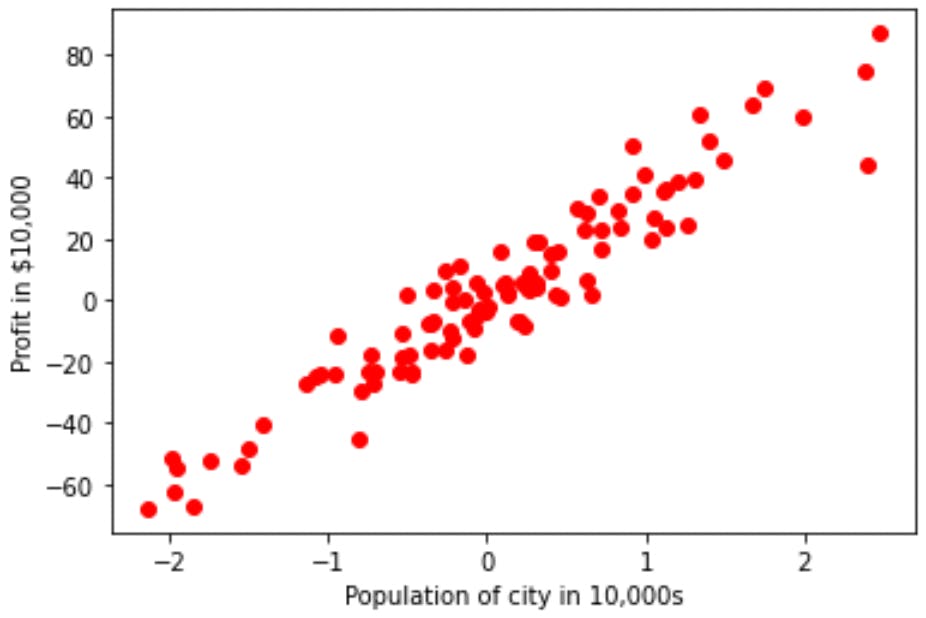
Testing on datasets
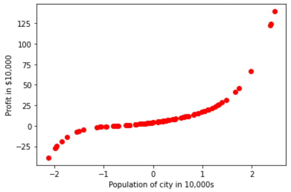
In this sub-section, we'll be using Sklearn's generated dataset for linear regression to see how our Linear Regression class is performing. Let's visulaize it on graph:
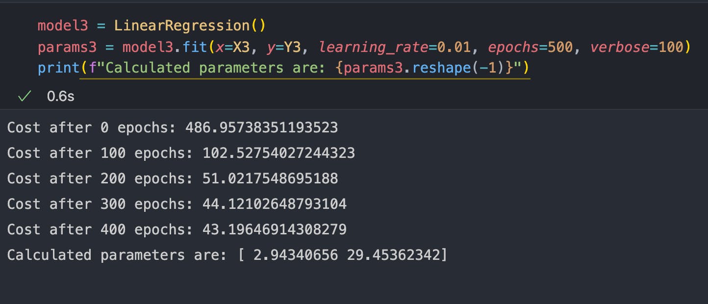
Let's create an instance of the LinearRegression class and fit this data on it for 500 epochs to get the optimal parameters for our hypothesis.
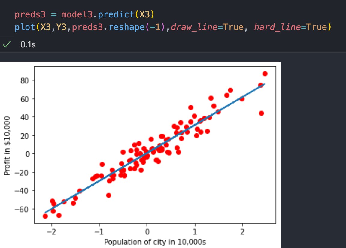
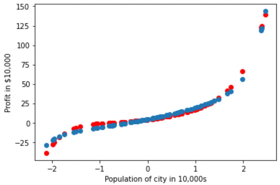
Okay, let's see how this hypothesis looks:
It fits nicely, but plotting the cost is a great way to assure that everything is working fine, let's do that. LinearRegression class had a property of cost_history and it stores the cost after each iteration, let's plot it:
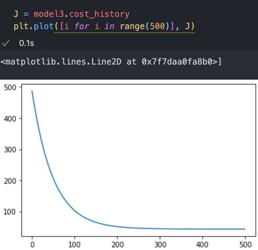
We can see that our cost function is always decreasing and it's a good sign to show that our model is working pretty good.
Before moving on to the next section and discussing Regularization, I want to demonstrate how we can also fit a curve instead of a straight line to a dataset, let's see it in the next sub-section.
Polynomial Regression
We basically going to take the generated dataset for linear regression from sklearn and apply some transformation to it to make it non-linear.
Note: For detailed code implementation I recommend you to go through the notebook from here since for the sake of learning I'm only showing a few code cells for verification
So what we did is generate the data from Sklearn's make_regression of 1 feature and a target column then apply the following transformation on it to make that data non-linear

and after applying to the dataset, it looks like:
Looks good we are able to introduce non-linearity but it'll be great if it also contains some noise samples, anyway let's start working on this non-linear dataset.
To make our linear regression predict a non-linear hypothesis we need to create more features (since we have only 1 here) from the features we already have. A popular way to create more features is to perform some polynomial functions on the original features one by one. For this example, we are going to make 6 different features from the original one:
We will be stacking these X1, X2, ..., X6 as features to make our final input/feature matrix X_. Now let's use this X_ matrix to predict the optimal curve.
The process of fitting and predicting is the same as shown in the previous section, or you can also refer to the notebook for better clarity.
It looks great, our algorithm is able to predict a fine non-linear boundary and it fits our training set very precisely. But there's a problem, we can see that our algorithm is performing very well on the training set and it's also possible that it won't work good on the data outside the training set. This is known as Overfitting and it leads to the lack of generality in the hypothesis.
We are going to address this problem using Regularization in the next section.
Regularization
With the help of Regularization, we can prevent the problem of overfitting from our algorithm. Overfitting occurs when the algorithm provides heavy parameters to some features according to the training dataset and hyperparameters. This makes those features dominant in the overall hypothesis and lead to a nice fit in the training set but not so good on the samples outside the training set.
The plan is to add the square of parameters by multiplying them with some big number (λ) to the cost function because our algorithms' main motive is to decrease the cost function so in this way algorithm will end up giving the small parameters just to cancel the effect addition of parameters by multiplying with a large number. So our final cost function gets modified to:
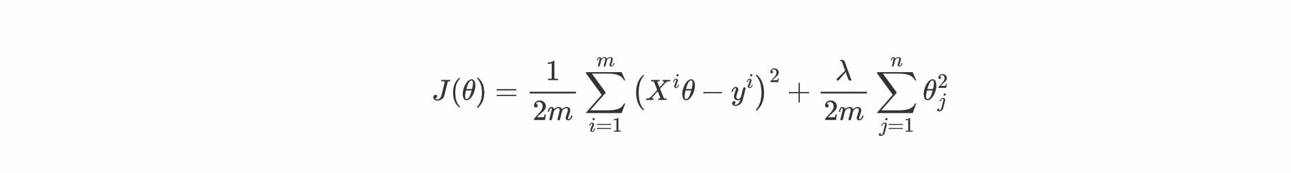
Note: We denote the bias term as θ0 and it's not needed to regularized the bias term that's why we are only considering only θ1 to θn parameters.
Since our cost function is changed that's why our formulas for gradients were also get affected. The new formula for the gradient are:
λ is known as a regularization parameter and it should be greater than 0. A large value of λ leads to underfitting and very small values lead to overfitting, so you need to pick the right one for your dataset by iterating on some sample values.
Let's implement the Regularization by modifying our LinearRegression class. We only need to modify the calculate_cost method because only this method is responsible for calculating both cost and gradients. The modified version is shown below:
class LinearRegression:
    def __init__(self) -> None:
        self.X = None
        self.Y = None
        self.parameters = None
        self.cost_history = []
        self.mu = None
        self.sigma = None

    def calculate_cost(self, lambda_=0):
        """
        Returns the cost and gradients.
        parameters:
            lambda_ : value of regularization parameter (default is 0)

        Returns:
            cost : Caculated loss (scalar).
            gradients: array containing the gradients w.r.t each parameter

        """
        m = self.X.shape[0]

        y_hat = np.dot(self.X, self.parameters)
        y_hat = y_hat.reshape(-1)
        error = y_hat - self.Y

        cost = (np.dot(error.T, error) + lambda_*np.sum((self.parameters)**2))/(2*m)

        gradients = np.zeros(self.X.shape[1])

        for i in range(self.X.shape[1]):
            gradients[i] = (np.mean(error * self.X[:,i]) + (lambda_*self.parameters[i])/m)

        return cost, gradients


    def init_parameters(self):
        """
        Initialize the parameters as array of 0s
        parameters: None

        Returns:None

        """
        self.parameters = np.zeros((self.X.shape[1],1))


    def feature_normalize(self):
        """
        Normalize the samples.
        parameters:
            X : input/feature matrix

        Returns:
            X_norm : Normalized X.

        """
        X_norm = self.X.copy()
        mu = np.mean(self.X, axis=0)
        sigma = np.std(self.X, axis=0)

        self.mu = mu
        self.sigma = sigma

        for n in range(self.X.shape[1]):
            X_norm[:,n] = (X_norm[:,n] - mu[n]) / sigma[n]
        return X_norm

    def fit(self, x, y, learning_rate=0.01, epochs=500, lambda_=0, is_normalize=True, verbose=0):
        """
        Iterates and find the optimal parameters for input dataset
        parameters:
            x : input/feature matrix
            y : target matrix
            learning_rate: between 0 and 1 (default is 0.01)
            epochs: number of iterations (default is 500)
            is_normalize: boolean, for normalizing features (default is True)
            verbose: iterations after to print cost

        Returns:
            parameters : Array of optimal value of weights.

        """
        self.X = x
        self.Y = y
        self.cost_history = []
        if self.X.ndim == 1: # adding extra dimension, if X is a 1-D array
            self.X = self.X.reshape(-1,1)
            is_normalize = False
        if is_normalize:
            self.X = self.feature_normalize()
        self.X = np.concatenate([np.ones((self.X.shape[0],1)), self.X], axis=1)
        self.init_parameters()

        for i in range(epochs):
            cost, gradients = self.calculate_cost(lambda_=lambda_)
            self.cost_history.append(cost)
            self.parameters -= learning_rate * gradients.reshape(-1,1)

            if verbose:
                if not (i % verbose):
                    print(f"Cost after {i} epochs: {cost}")

        return self.parameters


    def predict(self,x, is_normalize=True):
        """
        Returns the predictions after fitting.
        parameters:
            x : input/feature matrix

        Returns:
            predictions : Array of predicted target values.

        """
        x = np.array(x, dtype=np.float64) # converting list to numpy array
        if x.ndim == 1:
            x = x.reshape(1,-1)
        if is_normalize:
            for n in range(x.shape[1]):
                x[:,n] = (x[:,n] - self.mu[n]) / self.sigma[n]
        x = np.concatenate([np.ones((x.shape[0],1)), x], axis=1)
        return np.dot(x,self.parameters)
Now we have our regularized version of the LinearRegression class. Let's address the previous problem of overfitting on polynomial regression by using a set of values for λ to pick the right one.
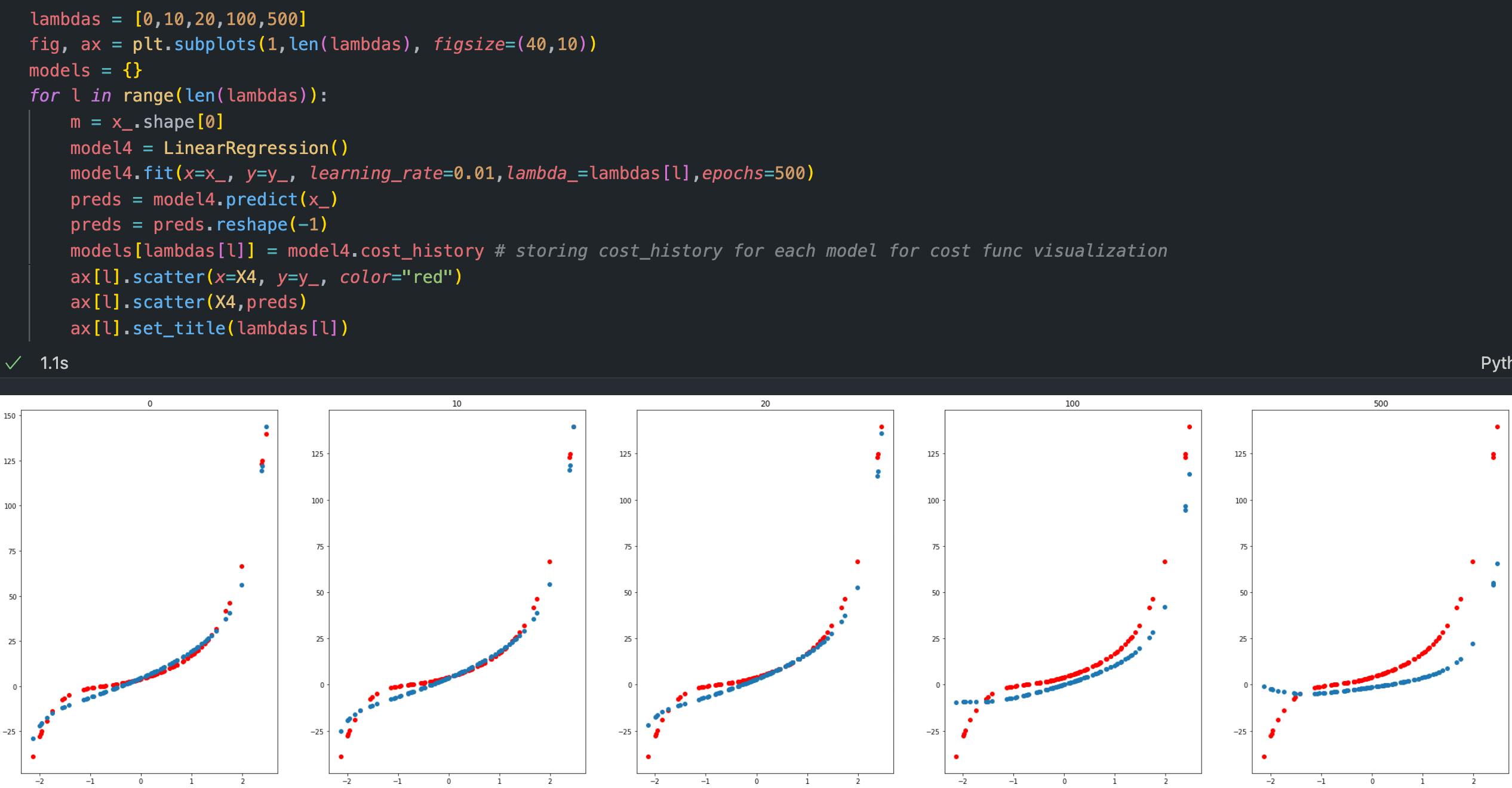
From the plots, I think that λ = 10 and λ = 20 looks good. We can see that as we increase the values of λ, our algorithm starts to perform even worst on the training set and leads to Underfitting. So it gets really important to select the right value of λ for our dataset.
Conclusion
Great work everyone, we successfully learnt and implemented Linear Regression using Gradient Descent. There are a few things that we need to keep in our mind that this optimizing algorithm requires more hyperparameters than the Normal equation that we learnt in the previous article but irrespective of that, gradient descent works efficiently on large datasets covering the drawback of the Normal equation method.
In the next article we'll be learning our first supervised classification algorithm known as Logistic Regression and going to understand how Regularization prevents overfitting there.
I hope you have learnt something new, for more updates on upcoming articles get connected with me through Twitter and stay tuned for more. Till then enjoy your day and keep learning.